ESC Calibration
-
Hello,
I am trying to calibrate ESC on VOXL2. I am using 1804-2800kv motors. When I runvoxl-esc-calibrate.pyfor each motors, I got some params.# Motor 1 pwm_vs_rpm_curve_a0 = 112.878194918 pwm_vs_rpm_curve_a1 = 0.336081465707 pwm_vs_rpm_curve_a2 = 7.53669159958e-06 # Motor 2 pwm_vs_rpm_curve_a0 = 35.6265065345 pwm_vs_rpm_curve_a1 = 0.37353561309 pwm_vs_rpm_curve_a2 = 2.9479165331e-06 # Motor 3 pwm_vs_rpm_curve_a0 = 132.362831923 pwm_vs_rpm_curve_a1 = 0.3256003514 pwm_vs_rpm_curve_a2 = 8.8413818561e-06 # Motor 4 pwm_vs_rpm_curve_a0 = -98.2189291548 pwm_vs_rpm_curve_a1 = 0.405821707061 pwm_vs_rpm_curve_a2 = 7.1523119742e-07But I know that in order to use VOXL-ESC parameters in the XML file, I need to put only one value. I put 4 sets of parameters for each motor, how do I make them into one parameter set?
First, please make sure that you are running the calibration with propellers installed (and use safety precautions).
Next, if you are doing several calibration tests (which sometimes makes sense) and want to use an average value, you have to be a little careful. Keep in mind that you cannot just average four a0 values and use it for a0_average (and so on). Also, even though the a0, a1, a2 numbers may look different, it is difficult to just look at the numbers and see how similar or different the curves are - the answer is to plot them.
I have written a short script to plot your four results using python. You can run it and take a look (first you may need to install
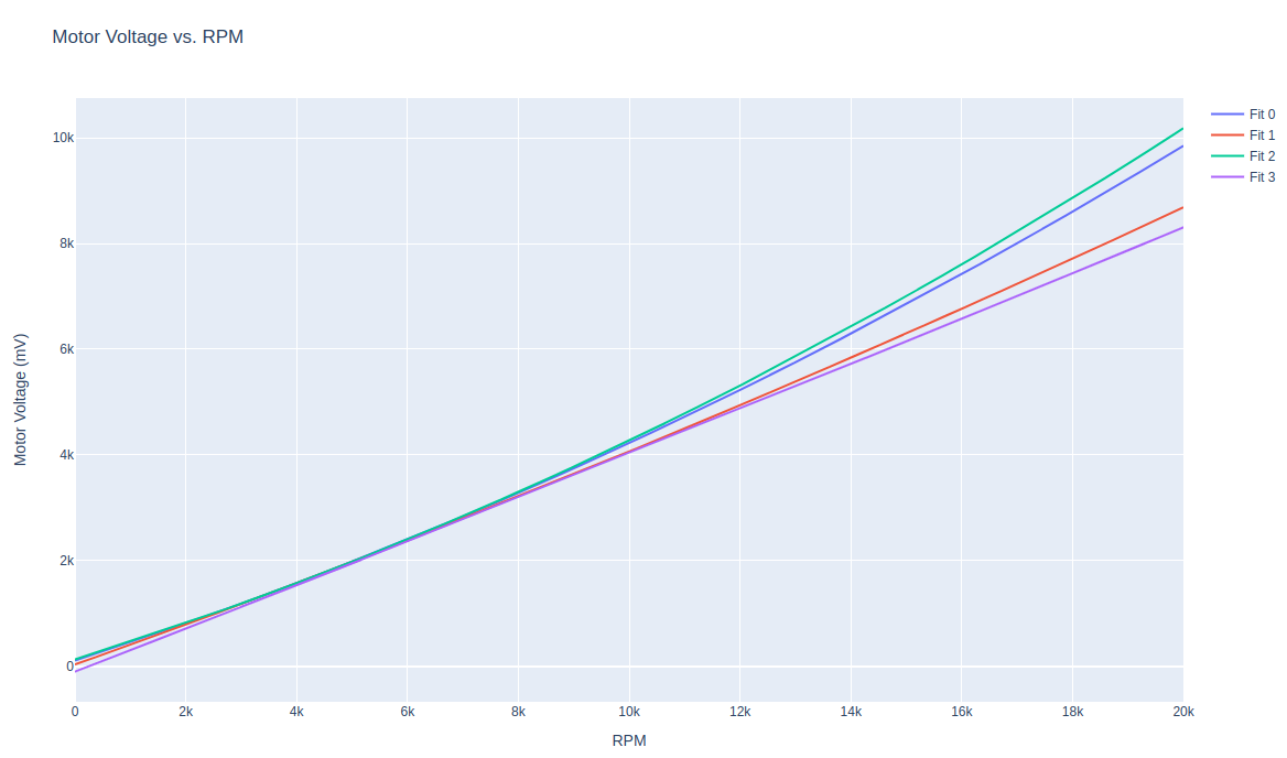
numpyandplotlypython packages usingpip3 install numpy plotly.import numpy as np import plotly.graph_objects as go rpms = np.arange(0,20000) #rpm range for the quadratic fit cals = [] fits = [] cals.append([7.53669159958e-06, 0.336081465707, 112.878194918]) cals.append([2.9479165331e-06, 0.37353561309, 35.6265065345]) cals.append([8.8413818561e-06, 0.3256003514, 132.362831923]) cals.append([7.1523119742e-07, 0.405821707061, -98.2189291548]) fig = go.Figure() for idx in range(len(cals)): fit = np.polyval(cals[idx], rpms) fits.append(fit) fig.add_trace(go.Scatter(x=rpms, y=fits[idx], name='Fit %d'%idx)) fig.update_layout(title='Motor Voltage vs. RPM') fig.update_xaxes(title_text="RPM") fig.update_yaxes(title_text="Motor Voltage (mV)") fig.show()The resulting plot looks like below, the four plots are not quite the same. But i have a feeling you might not have used propellers on during calibration? please confirm.
-
A Alex Kushleyev referenced this topic on
-
First, please make sure that you are running the calibration with propellers installed (and use safety precautions).
Next, if you are doing several calibration tests (which sometimes makes sense) and want to use an average value, you have to be a little careful. Keep in mind that you cannot just average four a0 values and use it for a0_average (and so on). Also, even though the a0, a1, a2 numbers may look different, it is difficult to just look at the numbers and see how similar or different the curves are - the answer is to plot them.
I have written a short script to plot your four results using python. You can run it and take a look (first you may need to install
numpyandplotlypython packages usingpip3 install numpy plotly.import numpy as np import plotly.graph_objects as go rpms = np.arange(0,20000) #rpm range for the quadratic fit cals = [] fits = [] cals.append([7.53669159958e-06, 0.336081465707, 112.878194918]) cals.append([2.9479165331e-06, 0.37353561309, 35.6265065345]) cals.append([8.8413818561e-06, 0.3256003514, 132.362831923]) cals.append([7.1523119742e-07, 0.405821707061, -98.2189291548]) fig = go.Figure() for idx in range(len(cals)): fit = np.polyval(cals[idx], rpms) fits.append(fit) fig.add_trace(go.Scatter(x=rpms, y=fits[idx], name='Fit %d'%idx)) fig.update_layout(title='Motor Voltage vs. RPM') fig.update_xaxes(title_text="RPM") fig.update_yaxes(title_text="Motor Voltage (mV)") fig.show()The resulting plot looks like below, the four plots are not quite the same. But i have a feeling you might not have used propellers on during calibration? please confirm.
@Alex-Kushleyev
It seems that when I run the script once, it only calibrates for one motor. So I ran the script 4 times to calibrate 4 motors. The motors spinned when I ran each script. Is there something I'm doing wrong?
I ran that script inside the drone, so I commented out the code to draw the plot. -
@Alex-Kushleyev
It seems that when I run the script once, it only calibrates for one motor. So I ran the script 4 times to calibrate 4 motors. The motors spinned when I ran each script. Is there something I'm doing wrong?
I ran that script inside the drone, so I commented out the code to draw the plot.@dlee , the calibration script indeed only spins one motor at a time, by design. Can you please confirm that you calibrated with propellers on?
-
@dlee , the calibration script indeed only spins one motor at a time, by design. Can you please confirm that you calibrated with propellers on?
-
@Alex-Kushleyev Yes, I calibrated with propellers on.
Got it. Can you tell me what was the maximum rpm reached during the calibration? I think i may have used too high rpm in the plot.
-
Got it. Can you tell me what was the maximum rpm reached during the calibration? I think i may have used too high rpm in the plot.
-
@Alex-Kushleyev Maximum RPM was reached at 13,000. I am using 2800kv motors.
Thanks. If you look at the plot at 13K rpm, the plots look much closer together. Also please note that there are two curves that are close together and another two that are also close together. I think they may correspond to CW and CCW rotating propellers. Sometimes the CW and CCW propellers are not exactly the same and could result in slightly different calibration..
I think for your initial testing you can use either of the calibration curves. However i am wondering whether your propellers are not symmetric CW and CCW.
You can also use a calibration that is an average. I will follow up soon how to calculate that.
-
@Alex-Kushleyev Is there any update?
@dlee , sorry for the delay.
Just to clarify, it is possible that your CW and CCW propellers are not exactly the same, therefore the CW and CCW motors are showing slightly different response to calibration. In this case we can calculate an average for this calibration and use that for all 4 motors. I modified the script to calculate the quadratic fit for all four calibration results together.
import numpy as np
import plotly.graph_objects as go

rpms = np.arange(0,13000) #rpm range for the quadratic fit

cals = []
fits = []
all_fits = []

#enter the calibration results from each motor
cals.append([7.53669159958e-06, 0.336081465707, 112.878194918])
cals.append([2.9479165331e-06,  0.37353561309,  35.6265065345])
cals.append([8.8413818561e-06,  0.3256003514,   132.362831923])
cals.append([7.1523119742e-07,  0.405821707061, -98.2189291548])

fig = go.Figure()

for idx in range(len(cals)):
    fit = np.polyval(cals[idx], rpms)
    fits.append(fit)
    fig.add_trace(go.Scatter(x=rpms, y=fits[idx], name='Fit %d'%idx))  #plot each fit

#create an array that contains points sampled from each curve
#and perform a polynomial fit on all the data to find the average
all_data = np.array(fits).flatten('C')
all_rpms = np.array([rpms,rpms,rpms,rpms]).flatten('C')

#evaluate the average poly fit
ply = np.polyfit(all_rpms, all_data, 2)
av_fit = np.polyval(ply, rpms)


#print the average fit coefficients
print('Average Fit coefficients:')
print('    pwm_vs_rpm_curve_a0 = ' + str(ply[2]))
print('    pwm_vs_rpm_curve_a1 = ' + str(ply[1]))
print('    pwm_vs_rpm_curve_a2 = ' + str(ply[0]))

#plot the average
fig.add_trace(go.Scatter(x=rpms, y=av_fit, name='Average Fit'))

#finalize and show the figure
fig.update_layout(title='Motor Voltage vs. RPM')
fig.update_xaxes(title_text="RPM")
fig.update_yaxes(title_text="Motor Voltage (mV)")
fig.show()
It results in the following plot and average coefficients. You can enter these coefficients into your custom esc parameters xml file.
Average Fit coefficients:
    pwm_vs_rpm_curve_a0 = 45.66215105517507
    pwm_vs_rpm_curve_a1 = 0.36025978431449995
    pwm_vs_rpm_curve_a2 = 5.01030529655002e-06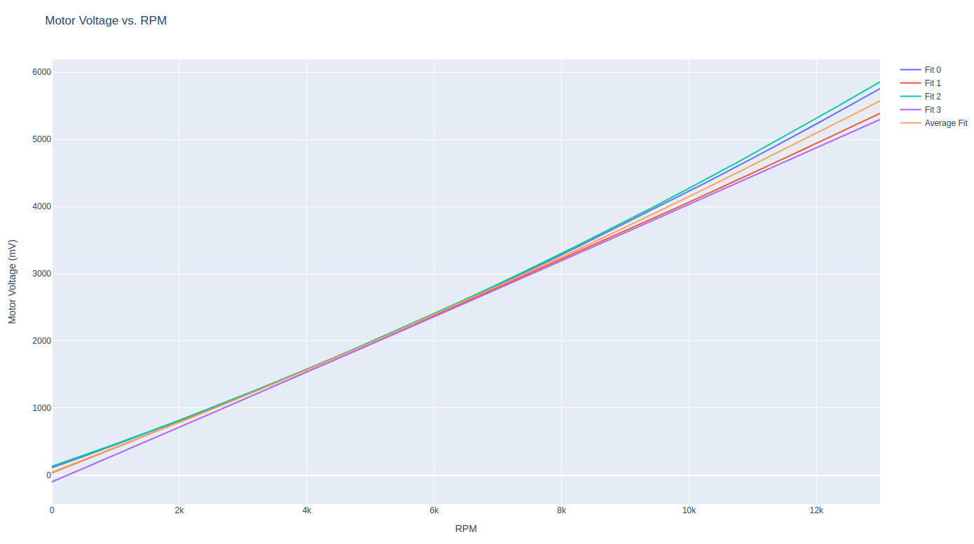
-
J John Nomikos 0 referenced this topic on
-
A Alexander Saunders referenced this topic on
Hello! It looks like you're interested in this conversation, but you don't have an account yet.
Getting fed up of having to scroll through the same posts each visit? When you register for an account, you'll always come back to exactly where you were before, and choose to be notified of new replies (either via email, or push notification). You'll also be able to save bookmarks and upvote posts to show your appreciation to other community members.
With your input, this post could be even better 💗
Register Login